OpenQEMIST-DMET with Microsoft Quantum Development Kit Libraries
This tutorial assumes users have installed:
the Microsoft .NET Core SDK, IQ# and the qsharp Python package
the openqemist Python package
A simple way to set up your environment is to use the docker image provided here. Otherwise, installation instructions can be found at https://github.com/1QB-Information-Technologies/openqemist.
1. Introduction
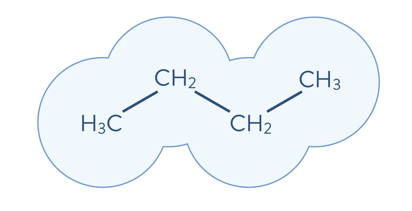
One of the main objectives of quantum chemistry calculations in the area of materials science is to solve the electronic structure problem, \(H\Psi=E\Psi\), as accurately as possible, in order to accelerate the materials design process. Here we solve the problem for the molecule shown below.
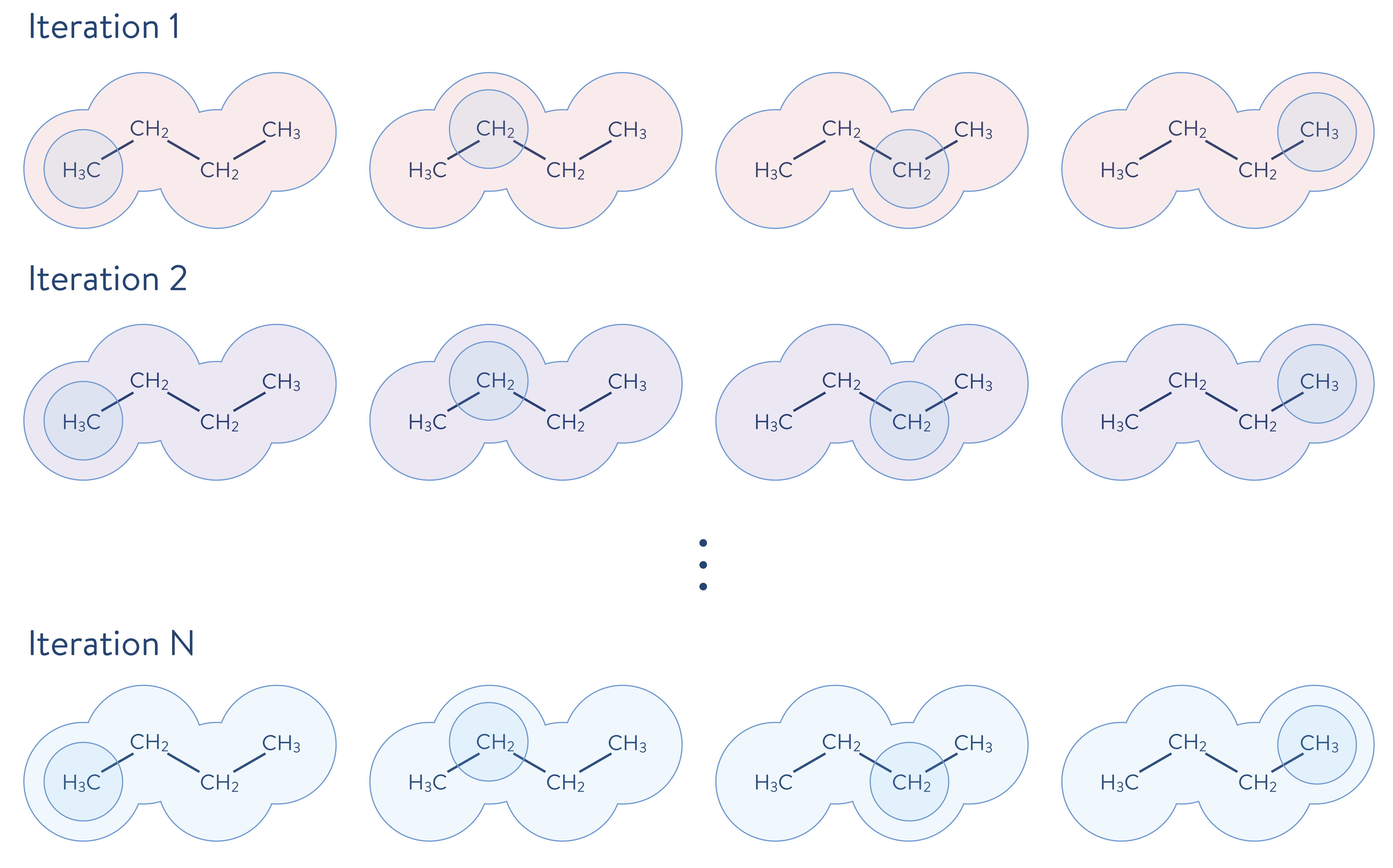
The computational cost for performing accurate calculations of the electronic structure of molecules, however, is usually very expensive. For example, the cost of performing the full CI calculation scales exponentially on a classical computer as the size of the system increases. Therefore, when we target large-sized molecules, those relevant for industry problems, it becomes essential to employ an appropriate strategy for reducing the computational cost, while maintaining accuracy, when performing electronic structure calculations. One such strategy is to decompose a molecular system into its constituent fragments and its environment, for each fragment independently, as appropriate for the problem. First, the environment outside of a fragment is calculated using a less-accurate method than will be used to calculate the electronic structure of a fragment. Then, the electronic structure problem for a given fragment is solved to a high degree of accuracy, which includes the quantum mechanical effects of the environment. The quantum mechanical description is updated (i.e., solved iteratively as shown below) by incorporating the just-performed highly accurate calculation. In the following schematic illustration, the molecule shown above is decomposed into fragments. Each molecular fragment CH\(_\mathrm{3}\) and CH\(_\text{2}\) are the fragments chosen for the electronic structure calculation, with the rest of the molecular system being the surrounding environment.
2. Density matrix embedding theory (DMET)
2-A. Theory
One successful decomposition approach is the DMET method\(^{1,2}\). The DMET method decomposes a molecule into fragments, and each fragment is treated as an open quantum system that is entangled with each of the other fragments, all taken together to be that fragment’s surrounding environment (or “bath”). In this framework, the electronic structure of a given fragment is obtained by solving the following Hamiltonian, by using a highly accurate quantum chemistry method, such as the full CI method or a coupled-cluster method.
The expression \(\sum_{mn} \left[ (rs|mn) - (rn|ms) \right] D^{\text{(mf)env}}_{mn}\) describes the quantum mechanical effects of the environment on the fragment, where \(D^{\text{(mf)env}}_{mn}\) is the mean-field electronic density obtained by solving the Hartree–Fock equation. The quantum mechanical effects from the environment are incorporated through the one-particle term of the Hamiltonian. The extra term \(\mu\sum_{r}^{\text{frag}} a_{r}^{\dagger}a_{r}\) ensures, through the adjustment of \(\mu\), that the number of electrons in all of the fragments, taken together, becomes equal to the total number of electrons in the entire system.
2-B. Performance of DMET
Here we provide examples of the performance results of DMET calculations (using classical simulation), employing some organic hydrocarbons (C\(_\mathrm{n}\)H\(_\mathrm{n}\)), below: tetrahedrane (C\(_\mathrm{4}\)H\(_\mathrm{4}\), top left), prismane (C\(_\mathrm{6}\)H\(_\mathrm{6}\), top centre), cubane (C\(_\mathrm{8}\)H\(_\mathrm{8}\), top right), cuneane (C\(_\mathrm{8}\)H\(_\mathrm{8}\), bottom left), pentaprismane (C\(_\mathrm{10}\)H\(_\mathrm{10}\), bottom centre), and diademane (C\(_\mathrm{10}\)H\(_\mathrm{10}\), bottom right). In these examples, each fragment consists of only one atom, thereby largely reducing the size of the electronic structure problem to be solved. Of the several electronic structure solvers used in DMET calculation we select the CCSD method (as it is the one most commonly used), the Meta-Löwdin as the localization\(^{3}\) scheme, and cc-pVDZ as the basis set. Visualizations are done with py3Dmol\(^{4}\).
import py3Dmol
view = py3Dmol.view(width=600,height=600,viewergrid=(2,3))

tetrahedrane = open('crd/tetrahedrane.xyz', 'r').read()
prismane = open('crd/prismane.xyz', 'r').read()
cubane = open('crd/cubane.xyz', 'r').read()
cuneane = open('crd/cuneane.xyz', 'r').read()
pentaprismane = open('crd/pentaprismane.xyz', 'r').read()
diademane = open('crd/diademane.xyz', 'r').read()

view.addModel(tetrahedrane,'xyz',viewer=(0,0))
view.addModel(prismane,'xyz',viewer=(0,1))
view.addModel(cubane,'xyz',viewer=(0,2))
view.addModel(cuneane,'xyz',viewer=(1,0))
view.addModel(pentaprismane,'xyz',viewer=(1,1))
view.addModel(diademane,'xyz',viewer=(1,2))

view.setStyle({'stick':{'colorscheme':'cyanCarbon'}})
view.zoomTo()
view.show()
You appear to be running in JupyterLab (or JavaScript failed to load for some other reason). You need to install the 3dmol extension:
jupyter labextension install jupyterlab_3dmol
2-B-a. Performance of DMET: Accuracy of calculation
This table shows the CCSD total energies (in a.u.), as well as the total energy difference (in kcal/mol) of DMET, MP2, B3LYP (DFT), and HF with respect to the reference CCSD value.
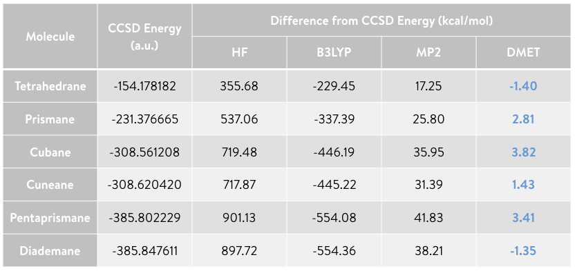
The total energy values of the DMET calculations agree with those obtained from CCSD, with only a small error, even though the fragment size in the DMET calculations is very small (i.e., there is only one atom per fragment). The calculations require only about 5% of the amplitudes (i.e., the parameters to be optimized) for tetrahedrane, and only 0.1% for pentaprismane, compared to performing a CCSD calculation of the full system. The number of terms of the Hamiltonian in DMET calculations is 1.5% and 0.05% of the full system for tetrahedrane and pentaprismane, respectively. A large amount of computational resources will therefore be saved without affecting the accuracy of the calculations.
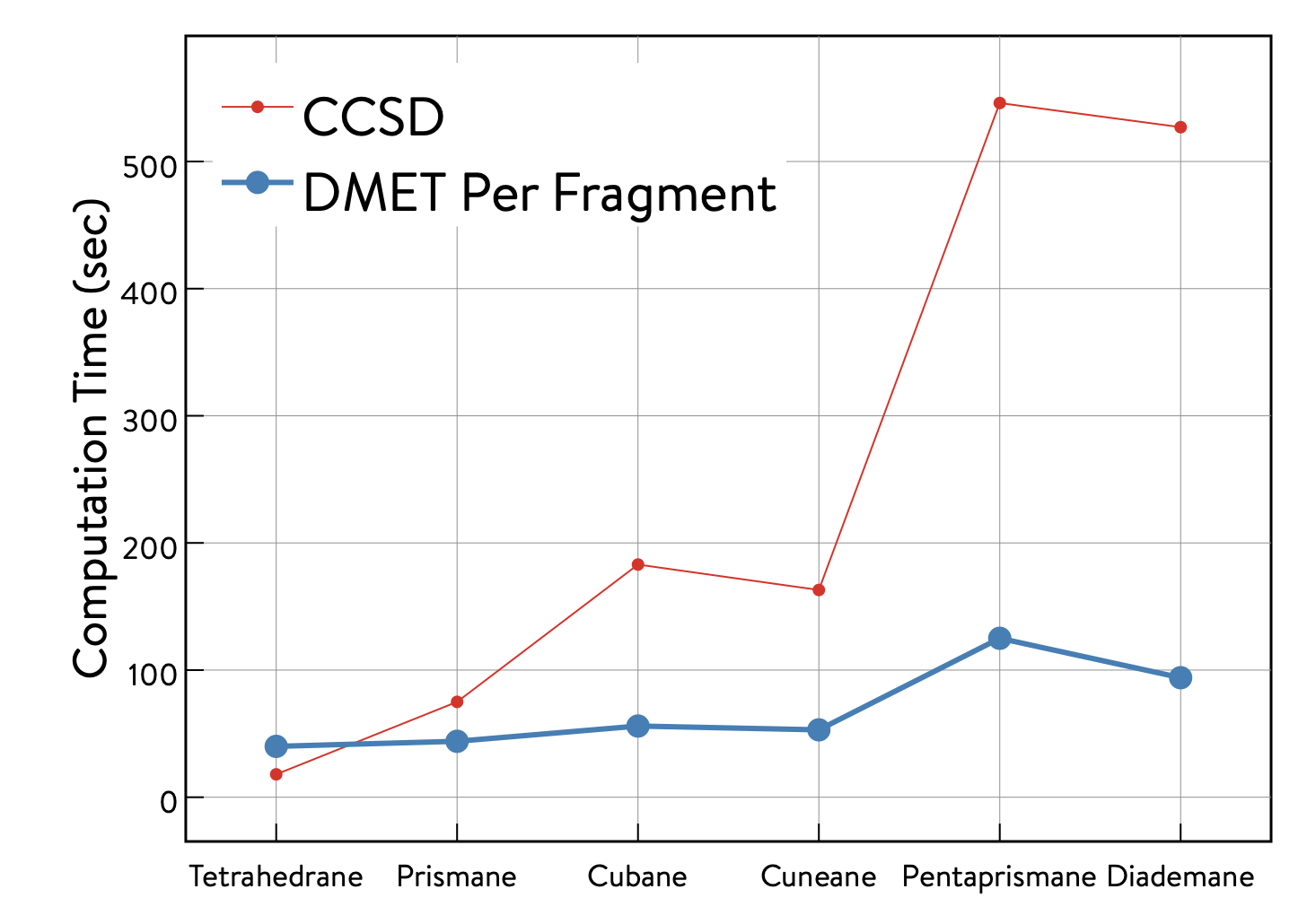
2-B-b. Performance of DMET: Computational time
The table below shows the computation time required for the full CCSD and DMET calculations, and the computation time of the DMET calculation per fragment (i.e., the DMET calculation time divided by the number of fragments used to decompose the molecule). Although the present examples are based on a serial implementation of DMET, the DMET calculation for each fragment can be trivially parallelized. Therefore, the DMET calculation time per fragment corresponds approximately to that of DMET executed in parallel.
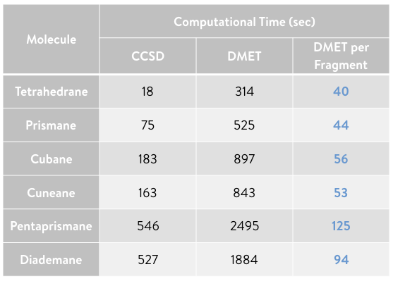
As shown in the plot, the computation time of the parallellized DMET calculation (blue) begins to demonstrate its advantage over the full CCSD calculation (red) as the molecular size increases.
3. OpenQEMIST-DMET sample calculation (classical simulation): A ring of 10 hydrogen atoms
3-A. Sample DMET script for OpenQEMIST
Here, we demonstrate how to perform DMET calculations using 1QBit’s OpenQEMIST (Quantum-Enabled Molecular ab Initio Simulation Toolkit) software package. Harnessing the power of emerging quantum computing technologies combined with state-of-the-art classical techniques, OpenQEMIST is able to deliver either state-of-the-art classical solutions or, with the flip of a switch, map a computationally challenging problem onto quantum computing architectures without the need for any additional programming, neither by a user nor a developer.
We have selected a ring of 10 hydrogen atoms as a simple example of a molecular system. The distance between adjacent hydrogen atoms has been set to 1\(~\)Å.
H10='''
H          1.6180339887          0.0000000000          0.0000000000
H          1.3090169944          0.9510565163          0.0000000000
H          0.5000000000          1.5388417686          0.0000000000
H         -0.5000000000          1.5388417686          0.0000000000
H         -1.3090169944          0.9510565163          0.0000000000
H         -1.6180339887          0.0000000000          0.0000000000
H         -1.3090169944         -0.9510565163          0.0000000000
H         -0.5000000000         -1.5388417686          0.0000000000
H          0.5000000000         -1.5388417686          0.0000000000
H          1.3090169944         -0.9510565163          0.0000000000
'''

view = py3Dmol.view(width=400,height=400)
view.addModel("10\n" + H10,'xyz',{'keepH': True})
view.setStyle({'sphere':{}})
view.setStyle({'model':0},{'sphere':{'colorscheme':'cyanCarbon','scale':'0.2'}})
view.zoomTo()
view.show()
You appear to be running in JupyterLab (or JavaScript failed to load for some other reason). You need to install the 3dmol extension:
jupyter labextension install jupyterlab_3dmol
Here we give the steps of a sample DMET calculation script.
Import DMET modules and localization schemes
from openqemist.problem_decomposition import DMETProblemDecomposition
from openqemist.problem_decomposition.electron_localization import iao_localization, meta_lowdin_localization
OpenQEMIST gives a user the ability to easily switch bewtween several electronic structure solvers, regardless of whether it is a classical or quantum solver. Here we present sample code using classical electronic structure solvers. In this open source version of OpenQEMIST, the Full CI and CCSD methods are currently available.
Import classical electronic structure solver modules
from openqemist.electronic_structure_solvers import FCISolver
from openqemist.electronic_structure_solvers import CCSDSolver
In OpenQEMIST, the inputs to all items of type “object” in OpenQEMIST are objects from the PySCF\(^{5}\) program. First we create the molecule object. Then we set up the OpenQEMIST objects.
Here we create a molecule object, and a problem decomposition object (a OpenQEMIST object), which problem decomposition techniques in OpenQEMIST require. The problem decomposition object holds an instance of an electronic structure solver, in this case the classical CCSD solver. We use the solver to perform the DMET simulation. An orbital localization technique needs to be defined to execute the DMET simulation. We employ the Meta-Löwdin localization method in this example DMET simulation. The orbital were depicted with VMD\(^{6}\).
Build molecule object (using PySCF) for DMET calculation
from pyscf import gto
mol = gto.Mole() # Instantiate the molecule class in PySCF
mol.atom = H10   # The coordinates of the atoms of the 10-hydrogen-atom ring are defined above
mol.basis = "minao" # Use "minao" as the basis set
mol.charge = 0 # Assign the charge of the molecule
mol.spin = 0 # Assign the spin of the molecule
mol.build() # Build the molecule object
<pyscf.gto.mole.Mole at 0x7faef51b7400>
Instantiate DMET class
dmet_solver = DMETProblemDecomposition()
Instantiate CCSD class
dmet_solver.electronic_structure_solver = CCSDSolver()
Select orbital localization technique (here Meta-Löwdin)
dmet_solver.electron_localization_method = meta_lowdin_localization
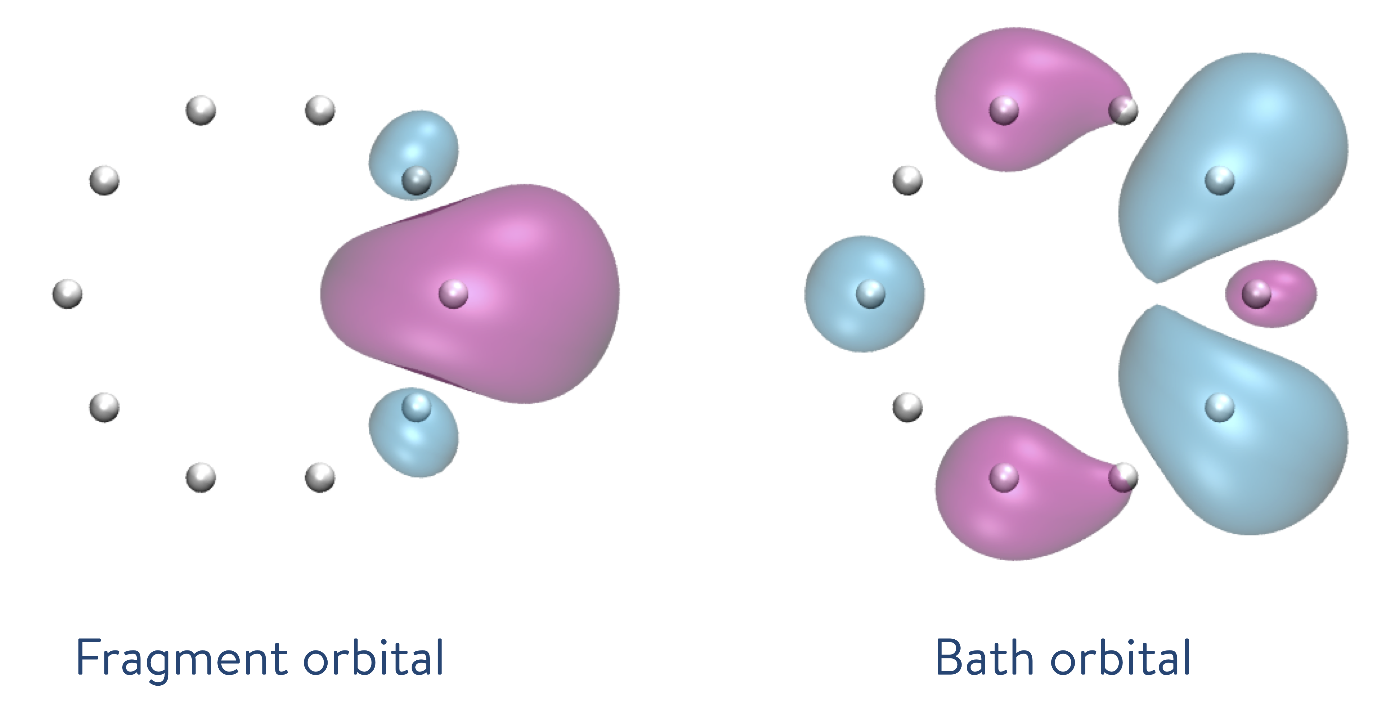
We perform a DMET calculation with one atom per fragment, with the localization of molecular orbitals being executed before entering the DMET loop. The resulting orbitals localized on each fragment are depicted here.
Perform DMET calculation
The “simulate” function takes two arguments: 1. the molecule object; 2. a list of the number of atoms each fragment has (i.e., in this case, 10 fragments, with one atom per fragment)
energy = dmet_solver.simulate(mol, [1,1,1,1,1,1,1,1,1,1])

print(energy)
-5.3675327924452745
3-B. Results of DMET calculation
This plot shows the potential energy curves of the ring of hydrogen atoms in atomic units (a.u.) for four methods.
After repeating the DMET calculations for the ring of hydrogen atoms by symmetrically stretching the distance between them, we obtain discrete sample points of the potential energy, which we plot alongside the curves of the other methods. The energy has been plotted as the energy per atom.
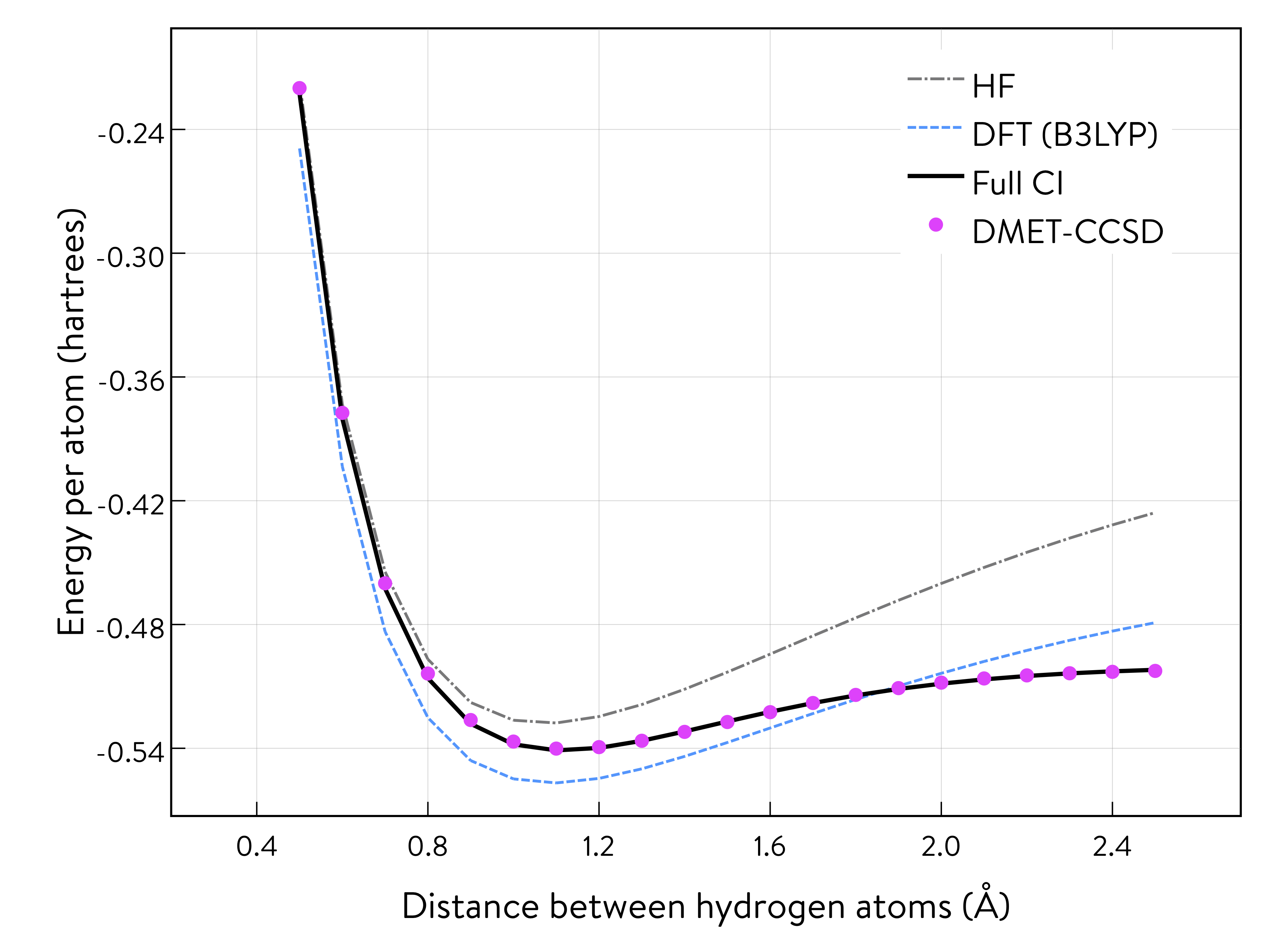
The results obtained from the DMET-CCSD method (using problem decomposition) are almost identical to those of the Full CI method (without using problem decomposition). When we decompose the ring of atoms into fragments, one of which includes only one hydrogen atom, the DMET method creates a fragment orbital (left: the single orbital distribution is shown in both pink and blue, with the colours depicting the phases) and the bath orbital (right: the single orbital distribution of the remaining nine hydrogen atoms is shown in both pink and blue, with the colours depicting the phases).
Then, the DMET Hamiltonian will consist of only two electrons and two (i.e., fragment and bath) orbitals. Therefore, the CCSD solver, which treats single- and double-excitations, will provide results equivalent to those of the Full CI solver. This is why the results of the DMET-CCSD and Full CI methods almost coincide.
The DMET calculations require only about 0.6% of the amplitudes compared to the CCSD calculation for the full system consisting of 10 hydrogen atoms. The number of Hamiltonian terms in the DMET calculation in the spacial orbital basis is only 20% (17% in the spin orbital basis) of the full system. A large amount of computational resources are saved while maintaining the same level of accuracy in the calculations.
4. DMET-VQE quantum simulation with Microsoft Quantum Development Kit Libraries
4-A. Sample script of DMET calculation combining OpenQEMIST and MS QDK 1: A ring of 10 hydrogen atoms
Here we describe how to perform DMET calculations using the variational quantum eigensolver (VQE) as the electronic structure solver. We use the UCCSD-VQE framework available in the Microsoft Quantum Development Kit libraries.\(^{7}\)
from openqemist.quantum_solvers.parametric_quantum_solver import ParametricQuantumSolver
from openqemist.quantum_solvers import MicrosoftQSharpParametricSolver
from openqemist.electronic_structure_solvers import VQESolver

vqe = VQESolver()
vqe.hardware_backend_type = MicrosoftQSharpParametricSolver
vqe.ansatz_type = MicrosoftQSharpParametricSolver.Ansatze.UCCSD

dmet = DMETProblemDecomposition()
dmet.electron_localization_method = meta_lowdin_localization
dmet.electronic_structure_solver = vqe
energy_vqe = dmet.simulate(mol, [1,1,1,1,1,1,1,1,1,1])
print(energy_vqe)
print(energy-energy_vqe)
-5.368762305205017
0.0012295127597425903
4-B. Results of DMET quantum simulation
The results of the DMET-CCSD calculation and those of the DMET-UCCSD-VQE method almost coincide. It has been reported\(^{8}\) that the UCCSD method performs better than the CCSD method; however, as discussed, both the CCSD and UCCSD solvers provide results equivalent to those of the Full CI solver.
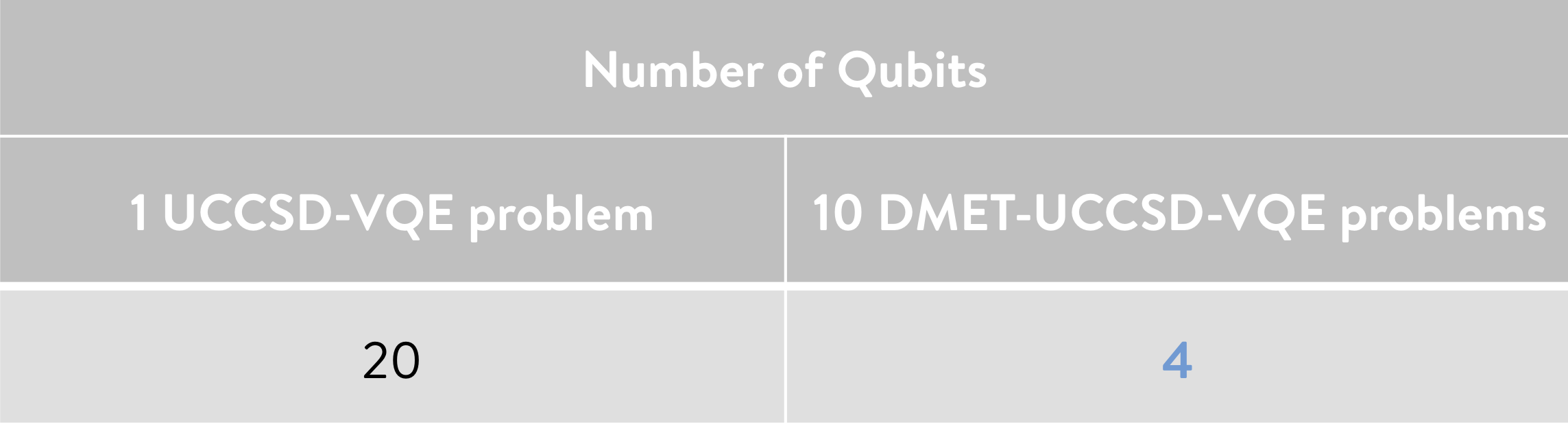
The DMET method decomposes the ring of 10 hydrogen atoms into 10 subproblems, each of which requires only four qubits to perform a quantum simulation, whereas the CCSD calculation of the full system requires 20 qubits, as shown.
4-C. Sample script of DMET calculation combining OpenQEMIST and MS QDK 2: Symmetric stretching of a ring of 10 hydrogen atoms
We repeat the DMET calculations for the ring of hydrogen atoms by symmetrically stretching the distance between the atoms.
energy_vqe_table = {}
for x in range(1,22):
    HH = 0.5+((x-1)*0.1)
    H10 = open('crd/h10_'+str(x)+'.xyz', 'r').readlines()[1:]
    H10 = ''.join(H10)

    mol = gto.Mole()
    mol.atom = H10
    mol.basis = "minao"
    mol.charge = 0
    mol.spin = 0
    mol.build()

    dmet = DMETProblemDecomposition()
    dmet.electron_localization_method = meta_lowdin_localization
    dmet.electronic_structure_solver = vqe
    energy_vqe = dmet_solver.simulate(mol, [1,1,1,1,1,1,1,1,1,1])
    energy_vqe_table.update({str(HH):energy_vqe})
Results of DMET quantum simulation 2
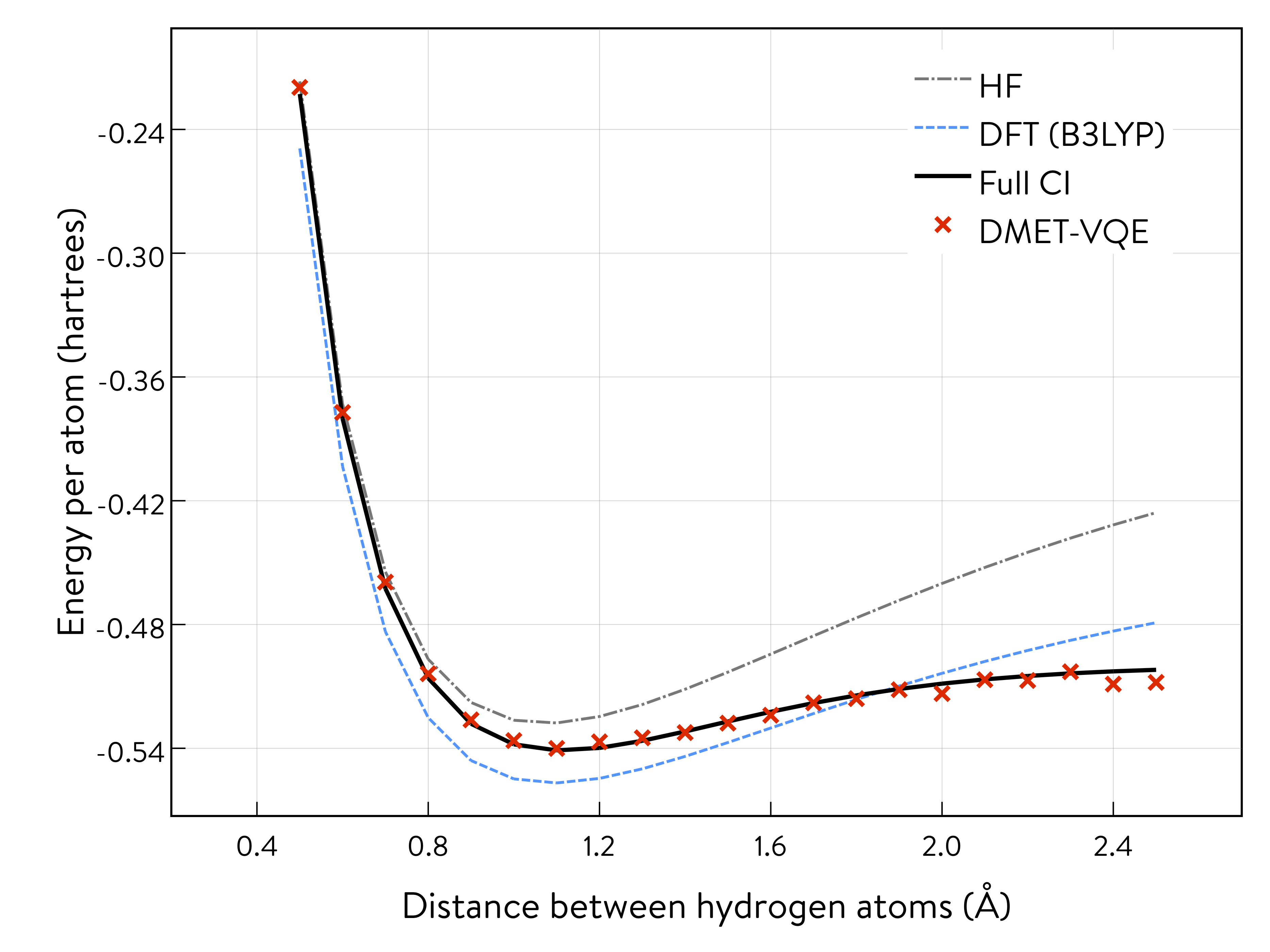
The potential energy curve of the DMET-VQE and FCI methods almost coincide, as shown.
It is also possible to estimate the quantum resources required based on the classical DMET calculations shown above. For pentaprismane, shown in an example classical simulation (see Section 2-B), DMET calculation requires 56 qubits, whereas 380 qubits are necessary for CCSD calculation of the full system. Thus, the DMET method can be a powerful tool for greatly reducing the computational resources needed.
5. References
Gerald Knizia and Garnet K.-L. Chan, “Density Matrix Embedding: A Simple Alternative to Dynamical Mean-Field Theory”, Phys. Rev. Lett., 109, 186404 (2012).
Sebastian Wouters, Carlos A. Jiménez-Hoyos, Qiming Sun, and Garnet K.-L. Chan, “A Practical Guide to Density Matrix Embedding Theory in Quantum Chemistry”, J. Chem. Theory Comput., 12, pp. 2706–2719 (2016).
Qiming Sun and Garnet K.-L. Chan, “Exact and Optimal Quantum Mechanics/Molecular Mechanics Boundaries”, J. Chem. Theory Comp., 10, 3784–3790 (2014).
py3Dmol. https://github.com/3dmol/3Dmol.js/tree/master/py3Dmol
Qiming Sun, Timothy C. Berkelbach, Nick S. Blunt, George H. Booth, Sheng Guo, Zhendong Li, Junzi Liu, James D. McClain, Elvira R. Sayfutyarova, Sandeep Sharma, Sebastian Wouters, and Garnet Kin‐Lic Chan, “PySCF: the Python‐based simulations of chemistry framework”, Wiley Interdiscip. Rev. Comput. Mol. Sci., 8, e1340 (2017).
William Humphrey, Andrew Dalke, and Klaus Schulten, “VMD – Visual Molecular Dynamics”, J. Molec. Graphics, 14, pp. 33–38 (1996). http://www.ks.uiuc.edu/Research/vmd
Guang Hao Low, Nicholas P. Bauman, Christopher E. Granade, Bo Peng, Nathan Wiebe, Eric J. Bylaska, Dave Wecker, Sriram Krishnamoorthy, Martin Roetteler, Karol Kowalski, Matthias Troyer, Nathan A. Baker, “Q# and NWChem: Tools for Scalable Quantum Chemistry on Quantum Computers”, arXiv:1904.01131 (2019).
Michael Kühn, Sebastian Zanker, Peter Deglmann, Michael Marthaler, and Horst Weiß, “Accuracy and Resource Estimations for Quantum Chemistry on a Near-term Quantum Computer”, arXiv:1812.06814 (2018).