The Variational Quantum Eigensolver (VQE)
This tutorial assumes users have installed:
the Microsoft .NET Core SDK, IQ# and the qsharp Python package
the openqemist Python package
A simple way to set up your environment is to use the docker image provided here. Otherwise, installation instructions can be found at https://github.com/1QB-Information-Technologies/openqemist.
1. A brief overview of the VQE algorithm
The Variational Quantum Eigensolver (VQE) [Peruzzo_et_al.,_2014, McClean_et_al.,_2015] has been introduced as a hybrid quantum–classical algorithm for simulating quantum systems. Some examples of quantum simulation using VQE include solving the molecular electronic Schrödinger equation and model systems in condensed matter physics (e.g., Fermi– and Bose–Hubbard models). In this notebook, we focus on VQE within the context of solving the molecular electronic structure problem for the ground-state energy of a molecular system. The second-quantized Hamiltonian of such a system, within the Born-Oppenheimer approximation, assumes the following form:
Here, \(h_{\text{nuc}}\) denotes the nuclear repulsion energy. The coefficients \(h^{p}_{q}\) and \(h^{pq}_{rs}\) are obtained by solving a mean-field problem. The Hamiltonian is then transformed into the qubit basis (e.g., Jordan–Wigner, Bravyi–Kitaev). This means that it is expressed entirely in terms of operators acting on qubits:
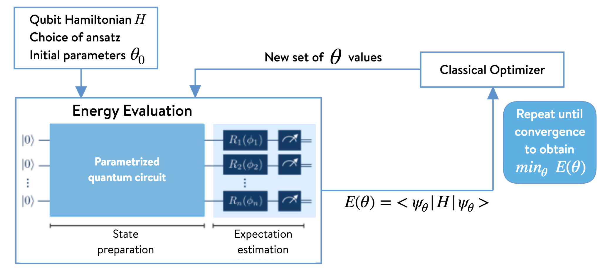
In this expression, the \(\sigma_p^\alpha\) are Pauli matrices (\(\alpha \in \{x,y,z\}\)), acting on the \(p\)-th qubit. We now consider a trial wavefunction ansatz \(\vert \Psi(\vec{\theta}) \rangle = U(\vec{\theta}) \vert 0 \rangle\) that depends on \(m\) parameters defining \(\vec{\theta}=(\theta_1, \theta_2, \ldots, \theta_m)\), which enter a unitary operator that acts on the reference (i.e., mean-field) state \(\vert 0 \rangle\). The variational principle dictates that we can minimize the expectation value of the Hamiltonian,
to determine the optimal set of variational parameters. The energy thus computed will be an upper bound to the true ground-state energy \(E_{\text{gs}}\). Once a suitable variational trial ansatz has been chosen (e.g., a unitary coupled-cluster ansatz, a heuristic ansatz), we must provide a suitable set of initial guess parameters. If our ansatz is written in according to the second quantization picture, we must also transform it into the qubit basis before proceeding. We must also apply other approximations (e.g., Trotter–Suzuki) to render it amenable for translation into a quantum circuit. The resulting qubit form of the ansatz can then be translated into a quantum circuit and, thus, able to be implemented on quantum hardware. Once the initial state has been prepared using a quantum circuit, energy measurements are performed using quantum hardware or an appropriate simulation tool. The energy value obtained is the sum of the measurements of the expectation values of each of the terms that contribute to the Hamiltonian (assuming the wavefunction has been normalized to unity):
The computed energy is then input to a classical optimizer in order to find a new set of variational parameters, which are then used to prepare a new state (i.e., a quantum circuit) on the quantum hardware. The process is repeated until convergence. The algorithm is illustrated below.
2. Computing the ground–state energy of H\(_{\text{2}}\) with UCCSD-VQE
The Microsoft Quantum Development Kit (QDK) provides a way to simulate quantum circuits on classical hardware and quantum processors. It uses the Microsoft Q# language, which was developed specifically to handle hybrid quantum–classical workflows.
The Quantum Development Kit chemistry library provides key functionalities for tackling problems in quantum chemistry. It is written in C#, and relies on Q# operations to implement various quantum algorithms. This is an open source GitHub repository that accepts suggestions and contributions.
Although users are able to write and call their own code in Q# and C#, this is not a requirement. This notebook uses Python exclusively. All the functionality needed to execute the example that follows can be accessed through the Quantum Development Kit Python interoperability package for python, qsharp, available on pip. Further details about this pip package are available at https://docs.microsoft.com/quantum/install-guide/python .
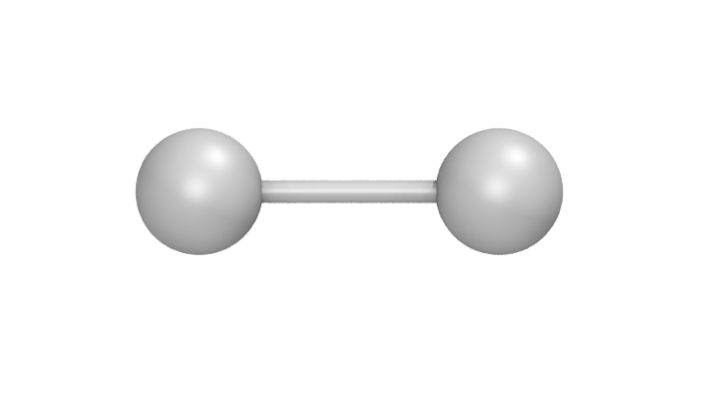
This section shows how these functionalities can be used to compute the ground state energy of H\(_{\mathrm{2}}\) (the simplest molecule) in a minimal basis set, using the unitary coupled-cluster ansatz with single and double excitations (UCCSD) and compare the results with the exact results obtained in this basis. A ball-stick model for H\(_\text{2}\) is shown below. The distance between the two hydrogen atoms is called the bond length, and its value is set to approximately 0.7414\(~\)Å in this section.
2-A The qsharp Python package
The cell below prepares the Q# environment and loads the useful
functionalities of the chemistry library through qsharp.chemistry.
This notebook later details how each of these play a role in this
implementation of VQE.
from qsharp.chemistry import load_broombridge, load_fermion_hamiltonian, load_input_state, encode
2-B Input data
Users need to provide quantities defining the target molecular system, such as the following:
one- and two-electron integrals
nuclear repulsion energy
The use of VQE requires to specify extra input, such as the following:
the type of ansatz desired (UCCSD, for example)
the values for initial variational parameters
an initial state (a reference wavefunction, such as the Hartree–Fock wavefunction)
The Broombridge
format,
created by Microsoft and PNNL, provides a way to store all the input
information in a human-readable .yaml file. Loading a pre-existing
Broombridge file containing the information of interest for the target
molecular system is the shortest way to get started with running VQE.
The qsharp.chemistry package allows Python packages to load and work
with the data stored in Broombridge files.
The following code snippet shows how to load existing data from a Broombridge file (here for H\(_\text{2}\) at a bond length of 0.7414), and explores the resulting data structure.
# C# Chemistry library :: Loading molecular data (electronic integrals, etc.) from Broombridge
filename = 'data/hydrogen_0.2.yaml'
broombridge_data =  load_broombridge(filename)
The data structure is easier to navigate when using a pretty-print application or a proper IDE.
It is worth mentioning that users do not need a Broombridge file describing the molecular system of interest in order to get started. They could, for example, compute and provide their own data at runtime using third-party libraries such as PySCF, and then be free to extract and overwrite the information in the data structures produced by reading any Broombridge file.
The instructions below show how users can read information stored in a data structure (writing to the data structure is just as straightforward).
# Retrieve basis set and geometry used to generate the input data
basis_set = broombridge_data.problem_description[0].basis_set
geometry = broombridge_data.problem_description[0].geometry

# Retrieve the nuclear repulsion and the one-electron integrals (Mulliken convention)
nuclear_repulsion = broombridge_data.problem_description[0].coulomb_repulsion['Value']
one_electron_integrals =  broombridge_data.problem_description[0].hamiltonian['OneElectronIntegrals']['Values']

print("nuclear_repulsion = ", nuclear_repulsion)
print("one_electron_integrals = ", one_electron_integrals)
nuclear_repulsion =  0.713776188
one_electron_integrals =  [([1, 1], -1.252477495), ([2, 2], -0.475934275)]
Note that users who are directly writing to the data structures should be aware that the Python interop relies on JSON serialization, and should use fundamental data types. They should make sure to pass lists instead of NumPy arrays, or to cast their integer and floating point values with the built-in int and float Python functions to avoid JSON serialization errors at runtime.
2-C Qubit Hamiltonian, UCCSD ansatz, and initial variational parameters
The following section shows how to prepare the qubit Hamiltonian (also referred to as the Pauli Hamiltonian) and access the information related to one of the available ansatz for VQE: UCCSD.
Note that the underlying data structures may change in the future. The
code cells below encourage users to print their content by directly
accessing the available fields, exposed by the dir built-in Python
function.
The fermionic Hamiltonian can be built using the chemistry library, and is returned to the Python context:
ferm_hamiltonian = broombridge_data.problem_description[0].load_fermion_hamiltonian()
print("ferm_hamiltonian ::", ferm_hamiltonian)
print(dir(ferm_hamiltonian))
ferm_hamiltonian :: <qsharp.chemistry.FermionHamiltonian object at 0x7f9774326550>
['__class__', '__delattr__', '__dict__', '__dir__', '__doc__', '__eq__', '__format__', '__ge__', '__getattribute__', '__gt__', '__hash__', '__init__', '__init_subclass__', '__le__', '__lt__', '__module__', '__ne__', '__new__', '__reduce__', '__reduce_ex__', '__repr__', '__setattr__', '__sizeof__', '__str__', '__subclasshook__', '__weakref__', 'add_terms', 'system_indices', 'terms']
A Broombridge file can contain suggestions of initial states to use to carry electronic computations of a molecule. In particular, they can be used by the UCCSD ansatz to store information about the initial state (i.e., the reference wavefunction) as well as initial values for the variational parameters and the spin-orbital excitations to whic they correspond.
Several initial states can be available and stored in a Broombridge file as a result of classical computations from libraries such as NWChem, for example. The user can specify which initial state to load with the following code snippet:
input_state = load_input_state(filename, "UCCSD |G>")
print("input_state ::", input_state)
print(dir(input_state))
input_state :: <qsharp.chemistry.InputState object at 0x7f9774230b00>
['Energy', 'MCFData', 'Method', 'SCFData', 'UCCData', '__class__', '__delattr__', '__dict__', '__dir__', '__doc__', '__eq__', '__format__', '__ge__', '__getattribute__', '__gt__', '__hash__', '__init__', '__init_subclass__', '__le__', '__lt__', '__module__', '__ne__', '__new__', '__reduce__', '__reduce_ex__', '__repr__', '__setattr__', '__sizeof__', '__str__', '__subclasshook__', '__weakref__']
Users can decide what excitations should be included in the ansatz and
how the values of variational parameters can be tied to specific
excitations, or enforce that a unique value should be tied to several
terms during the classical optimization later. The last entry in
inputstate[Superposition] is the initial state, here showing a
Hartree-Fock state, with the two lower orbitals filled with one electron
each.
The chemistry library can now build the qubit Hamiltonian with a transformation such as the Jordan–Wigner transformation.
jw_hamiltonian = encode(ferm_hamiltonian, input_state)
print("jw_hamiltonian :: \n", jw_hamiltonian)
jw_hamiltonian ::
 (4, ([([0], [0.17120128499999998]), ([1], [0.17120128499999998]), ([2], [-0.222796536]), ([3], [-0.222796536])], [([0, 1], [0.1686232915]), ([0, 2], [0.12054614575]), ([0, 3], [0.16586802525]), ([1, 2], [0.16586802525]), ([1, 3], [0.12054614575]), ([2, 3], [0.1743495025])], [], [([0, 1, 2, 3], [0.0, -0.0453218795, 0.0, 0.0453218795])]), (3, [((0.001, 0.0), [2, 0]), ((-0.001, 0.0), [3, 1]), ((-0.001, 0.0), [2, 3, 1, 0]), ((1.0, 0.0), [0, 1])]), -0.09883444600000002)
Please note that, currently, the underlying JordanWignerEncodingData
data structure from the chemistry library is also used to store the
initial state for UCCSD as well as the variational parameters
representing the one- and two-body amplitudes (specified as the third
entry of the resulting jw_hamiltonian tuple object). In the future,
the objects may be kept separate and thus the inputState field may
not be required to compute the qubit Hamiltonian. Users can, however,
retrieve the values of the variational parameters directly from the data
structure, with a function such as the following:
def get_var_params(jw_hamiltonian):
    """ Retrieve the values of variational parameters from the jw_hamiltonian object """
    _, _, input_state, _ = jw_hamiltonian
    _, var_params = input_state
    params = [param for ((param, _), _) in var_params]
    return params[:-1]

var_params = get_var_params(jw_hamiltonian)
print(var_params)
[0.001, -0.001, -0.001]
2-D Energy evaluation using the Q# quantum algorithms
The qsharp package can be used to directly call quantum algorithms written in Q#. These can be user defined, or come from one of the available Q# libraries.
The energy is computed as an expectation value
\(E(\theta) = \langle \Psi(\vec{\theta}) \vert \hat{H} \vert \Psi(\vec{\theta}) \rangle =\langle\hat{H}\rangle\),
which can be estimated by drawing many samples of the underlying
distribution (e.g., running the quantum circuit and measuring for each
sample). This approach is the one used on quantum hardware, and relies
on sampling to approach the expectation value, using the simulate
function. The accuracy of the expectation value, and therefore the
result of the energy evaluation, directly correlates with the number of
samples used. The fast frequency estimator provided in the QDK allows
for the approximation of the result for a very large number of samples
without incurring longer runtimes.
import qsharp

# It is possible to create a Python object to represent a
# Q# callable from the chemistry library
estimate_energy = qsharp.QSharpCallable("Microsoft.Quantum.Chemistry.JordanWigner.VQE.EstimateEnergy", "")

# The Q# operation can then be called through the simulate method
# A large number of samples is selected for high accuracy
energy = estimate_energy.simulate(jwHamiltonian=jw_hamiltonian, nSamples=1e18)

print("Energy evaluated at {0} : {1} \n".format(var_params, energy))
Energy evaluated at [0.001, -0.001, -0.001] : -1.1170458251864388
2-E Classical optimization
VQE is a quantum–classical hybrid algorithm that aims to compute \(E = \min_{\vec{\theta}} \: \langle \Psi(\vec{\theta}) \vert \hat{H} \vert \Psi(\vec{\theta}) \rangle\). This approach relies on solving an optimization problem, using a classical optimizer to tune the values of the variational parameters \(\{\theta_i\}_{i=1}^{m}\).
There are several Python libraries that provide implementations of
optimizers based on different heuristics, and SciPy is one that is
widely used. The optimizers in scipy.optimize have a common
interface that require users to provide the following:
A handle to a Python function to perform energy evaluations. It takes the variational parameters as its first input, leaving other parameters that are to be left out of the optimization process afterwards
Values for the initial parameters
Optional parameters used by our energy evaluation function, that should not be optimized
Optional parameters defining the behaviour and termination criteria for the chosen optimizer
The first item requires the user to provide a Python wrapper (here named
energy_eval_wrapper) with the expected signature, in order to call
the energy_evaluation operation available in the Quantum Development
Kit chemistry library. This wrapper requires the variational parameters
to be passed as a list or a NumPy array and, currently, an extra step is
needed to modify the data structure passed to the Q# context in order to
use the correct values (defined in set_var_params below).
def set_var_params(var_params, jw_hamiltonian):
    """ Set variational parameters stored in the JW data-structure to the desired values"""
    # Unpack data structure
    a1, a2, input_state, a3 = jw_hamiltonian
    b1, amps = input_state
    # Unpack and overwrite variational parameters
    new_amps = [((var_params[i], 0.0), amps[i][1]) for i in range(len(var_params))]
    new_amps.append(amps[-1])
    # Re-pack the data structure
    input_state = (b1, new_amps)
    jw_hamiltonian = (a1, a2, input_state, a3)
    return jw_hamiltonian
def energy_eval_wrapper(var_params, jw_hamiltonian, n_samples):
    """
        A wrapper whose signature is compatible with the use of scipy optimizers,
        calling the Q# energy_evalaution from the Microsoft Chemistry library
    """

    # NumPy arrays are currently not supported by the Python interops
    # This ensures that neither the user nor SciPy call the energy evaluation function with a NumPy array
    var_params = list(var_params)

    # Set the varational parameters to the right values in the jw_hamiltonian object
    jw_hamiltonian = set_var_params(var_params, jw_hamiltonian)

    # Estimate the energy
    energy = estimate_energy.simulate(jwHamiltonian=jw_hamiltonian, nSamples=1e18)

    print("Energy evaluated at {0} : {1} \n".format(var_params, energy))
    return energy
These two functions can then be used to run VQE. For simplicity, a specific optimizer from the SciPy library is used, with given hyperparameters such as tolerance or step size. Since accuracy of energy evaluation is correlated to the number of samples drawn, it is important to set it to a number large enough to guarantee that it is consistent with the optimizers convergence criteria, and to ensure the correct approximation of derivatives used by some optimizers. Setting a very large number of samples would solve this issue.
from scipy.optimize import minimize

def VQE(initial_var_params, jw_hamiltonian, n_samples):
    """ Run VQE Optimization to find the optimal energy and the associated variational parameters """

    opt_result = minimize(energy_eval_wrapper,
                          initial_var_params,
                          args=(jw_hamiltonian, n_samples),
                          method="COBYLA",
                          tol=0.000001,
                          options={'disp': True, 'maxiter': 200,'rhobeg' : 0.05})

    return opt_result
# Run VQE and print the results of the optimization process
# A large number of samples is selected for higher accuracy
opt_result = VQE(var_params, jw_hamiltonian, n_samples=1e18)
print(opt_result)
    fun: -1.137270414288908
  maxcv: 0.0
message: 'Optimization terminated successfully.'
   nfev: 57
 status: 1
success: True
      x: array([ 4.16719513e-06, -1.00637897e-05, -1.13066239e-01])
# Print difference with exact FCI value known for this bond length
fci_value = -1.1372704220924401
print("Difference with exact FCI value :: ", abs(opt_result.fun - fci_value))
Difference with exact FCI value :: 7.803532042771621e-09
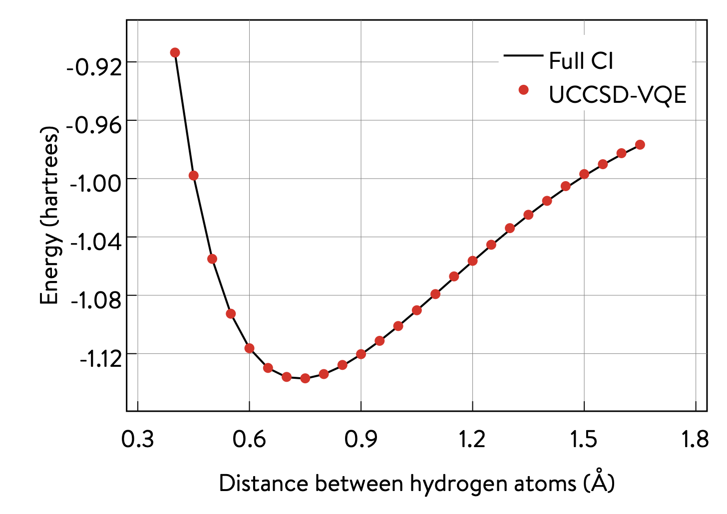
3 Potential energy surface of H\(_\text{2}\) with VQE, using the 1QBit OpenQEMIST package
The potential energy surface of this molecule can be obtained by plotting the energy of the system as a function of the distance between the hydrogen atoms.
This section shows how the 1QBit OpenQEMIST package allows users to run VQE without relying on an input Broombridge file, or worrying about modifying the data structures returned by the Python interop in the previous section. Users can directly provide the geometry and basis set of the target molecular system: OpenQEMIST computes the mean field and electronic integrals using PySCF, generates the UCCSD one- and two-body excitations, and provides good initial variational parameters using MP2 amplitudes.
OpenQEMIST provides several electronic structure solvers, such as VQE, FCI, and CCSD. This package can be used to compute the H\(_\text{2}\) bond dissociation curve using VQE, with Microsoft libraries, and compare it to the exact FCI values, computed on-the-fly. Running the code cells in this section should yield a plot that closely resembles the one below:
# Import the OpenQEMIST package from 1QBit and PySCF
import openqemist
import pyscf
import numpy as np
from pyscf import gto, scf
from openqemist.electronic_structure_solvers import VQESolver, FCISolver
from openqemist.quantum_solvers.parametric_quantum_solver import ParametricQuantumSolver
from openqemist.quantum_solvers import MicrosoftQSharpParametricSolver

# Iterate over different bond lengths
bond_lengths = np.arange(0.4, 1.7, 0.1)
energies_FCI, energies_VQE = [], []

for bond_length in bond_lengths:

    # Create molecule object with PySCF
    H2 = [['H',[ 0, 0, 0]], ['H',[0,0, bond_length]]]
    mol = gto.Mole()
    mol.atom = H2
    mol.basis = "sto-3g"
    mol.charge = 0
    mol.spin = 0
    mol.build()

    # Compute FCI energy with PySCF, for reference
    solver = FCISolver()
    energy = solver.simulate(mol)
    energies_FCI += [energy]

    # Compute energy with VQE, instantiating a VQESolver object using the UCCSD ansatz
    solver = VQESolver()
    solver.hardware_backend_type = MicrosoftQSharpParametricSolver
    solver.ansatz_type = MicrosoftQSharpParametricSolver.Ansatze.UCCSD
    energy = solver.simulate(mol)
    energies_VQE += [energy]
import matplotlib.pyplot as plt
%matplotlib inline

plt.plot(bond_lengths, energies_FCI, color = 'black', label='Full CI')
plt.plot(bond_lengths, energies_VQE, 'ro', label='UCCSD-VQE')
plt.title("Potential energy surface of H2")
plt.xlabel("Distance between hydrogen atoms (angstroms)")
plt.ylabel("Energy (hartrees)")
plt.legend()
<matplotlib.legend.Legend at 0x7f9735d7f048>